
You’ve probably heard that you need 1,000, 10,000, or even 100,000 physical qubits to build a logical qubit. These numbers are decent rules of thumb, but in practice it really depends: you have to figure it out for each unique situation.
Figuring this out is known as estimating the overhead.
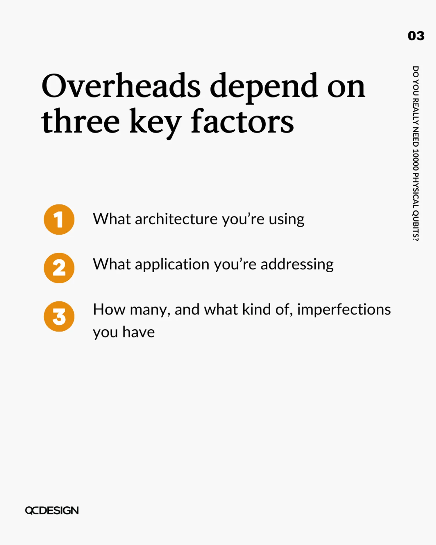
The overhead depends on three things: the architecture you’re using, the application you’re addressing, and the imperfections in your system.
Let’s work through each one of these.
The architecture you’re using
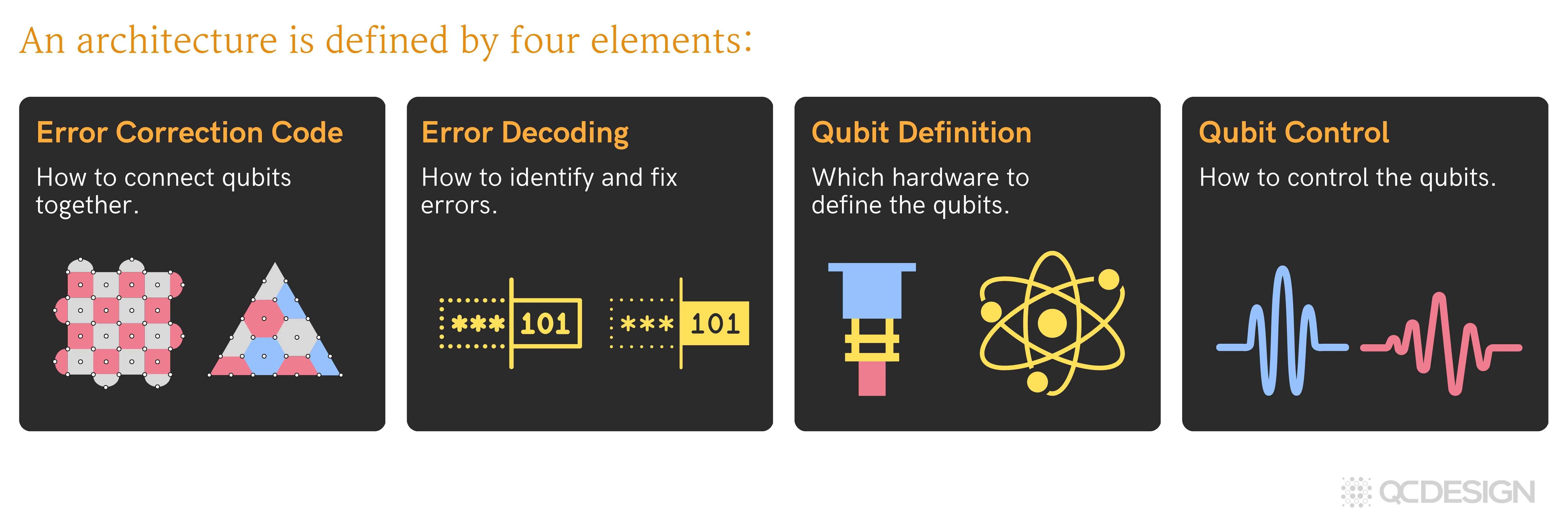
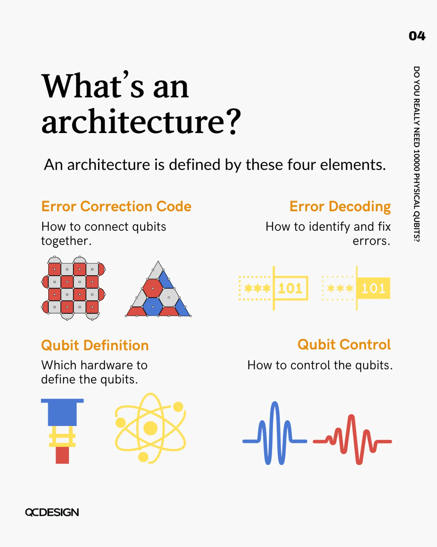
An architecture is defined by four elements:
- Error correction code: how to connect qubits together.
- Error decoding: how to identify and fix errors.
- Qubit definition: which hardware to define the qubits.
- Qubit control: how to control the qubits.
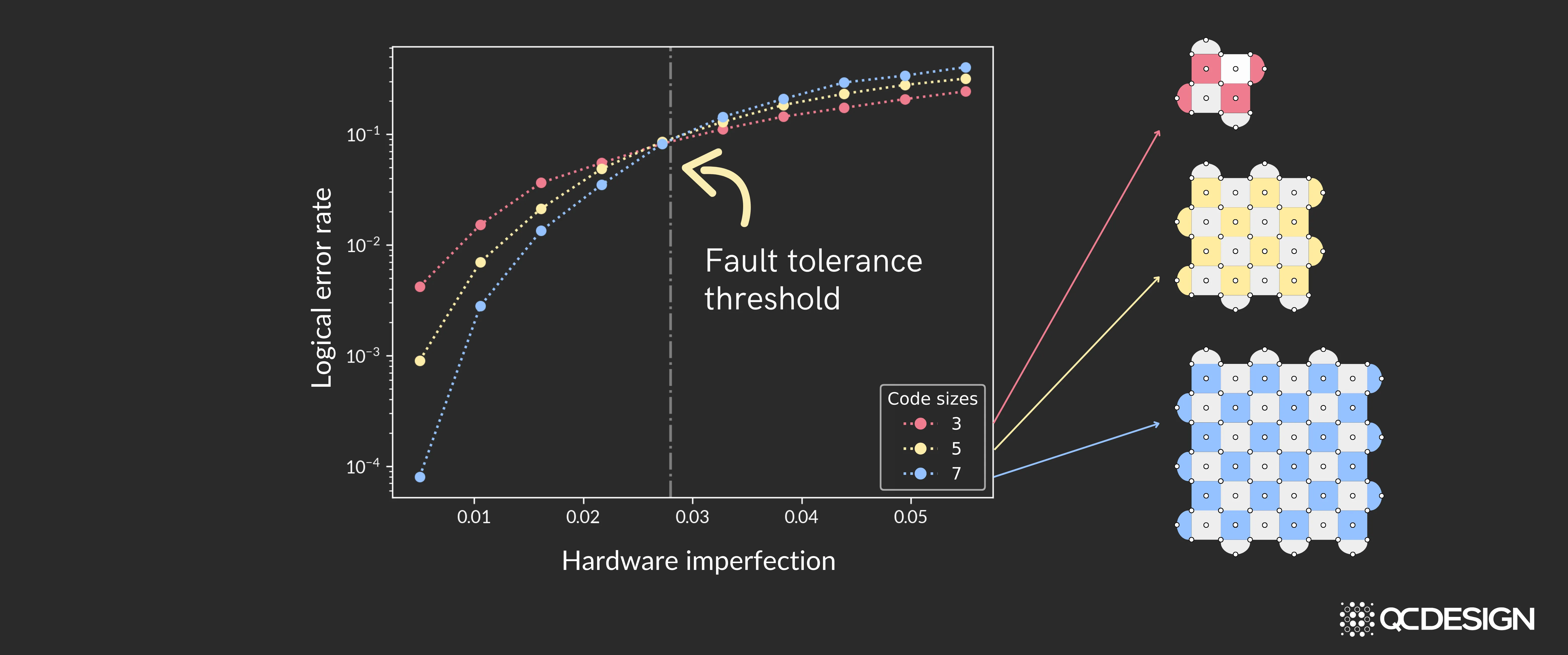
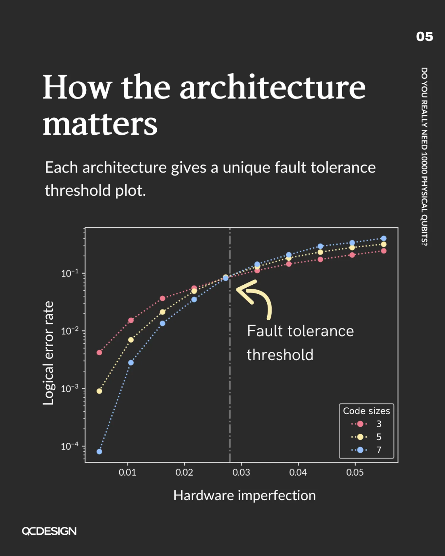
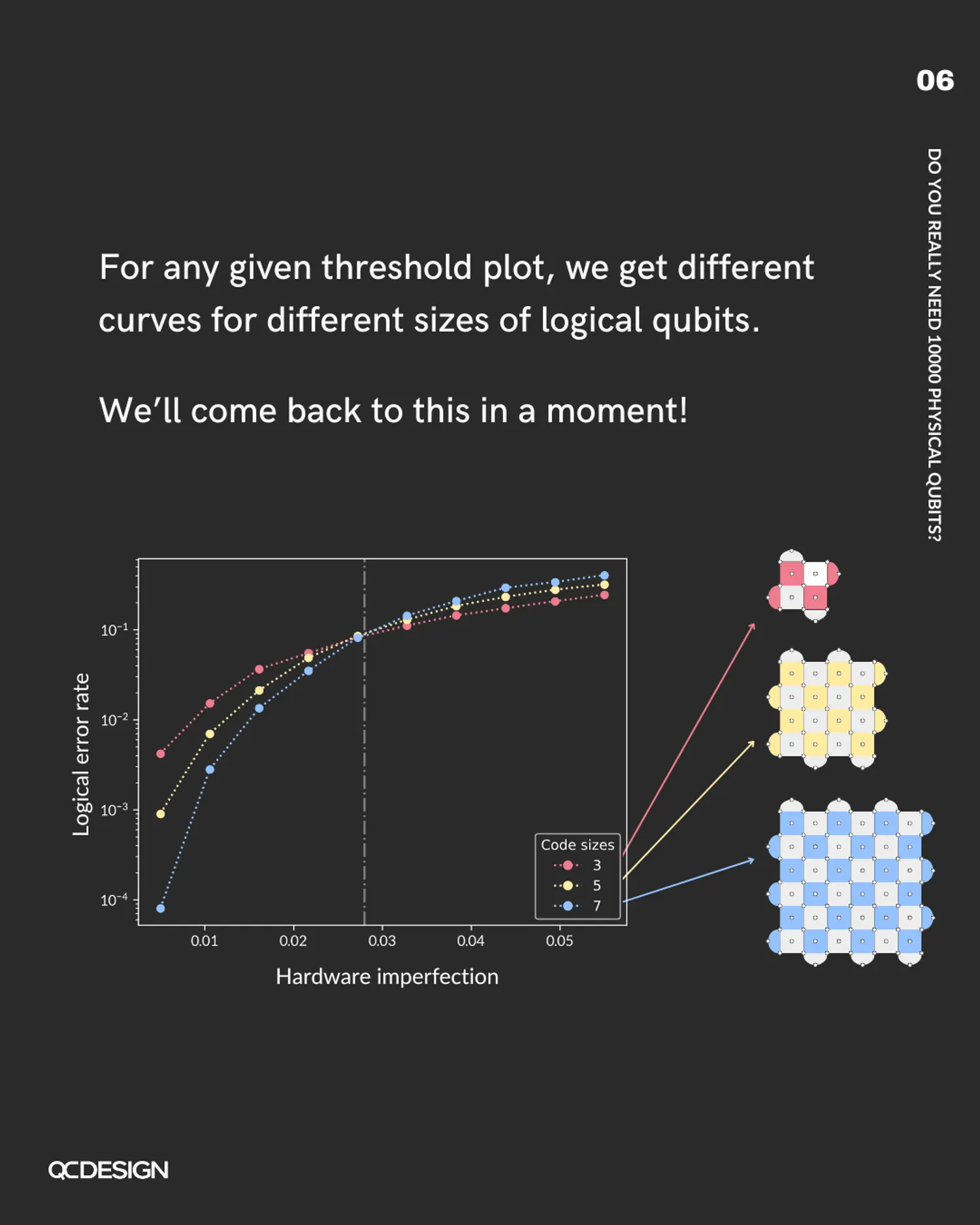
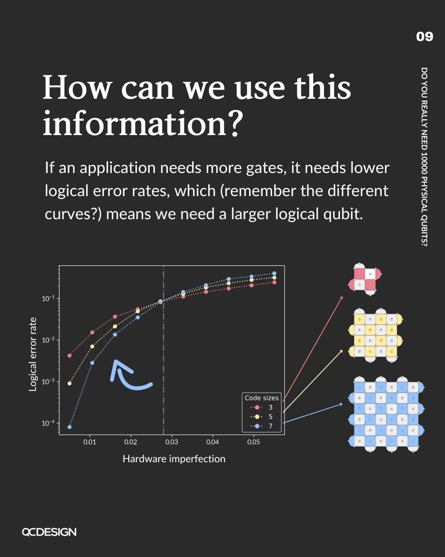
Each architecture gives a unique fault tolerance threshold plot, which defines a unique fault tolerance threshold (see arrow below). For any given plot, the curves differ depending on the size of the logical qubit. In the figure below, we see curves for logical qubits of code-sizes 3, 5, and 7. We’ll come back to this in a moment.
The application you’re addressing
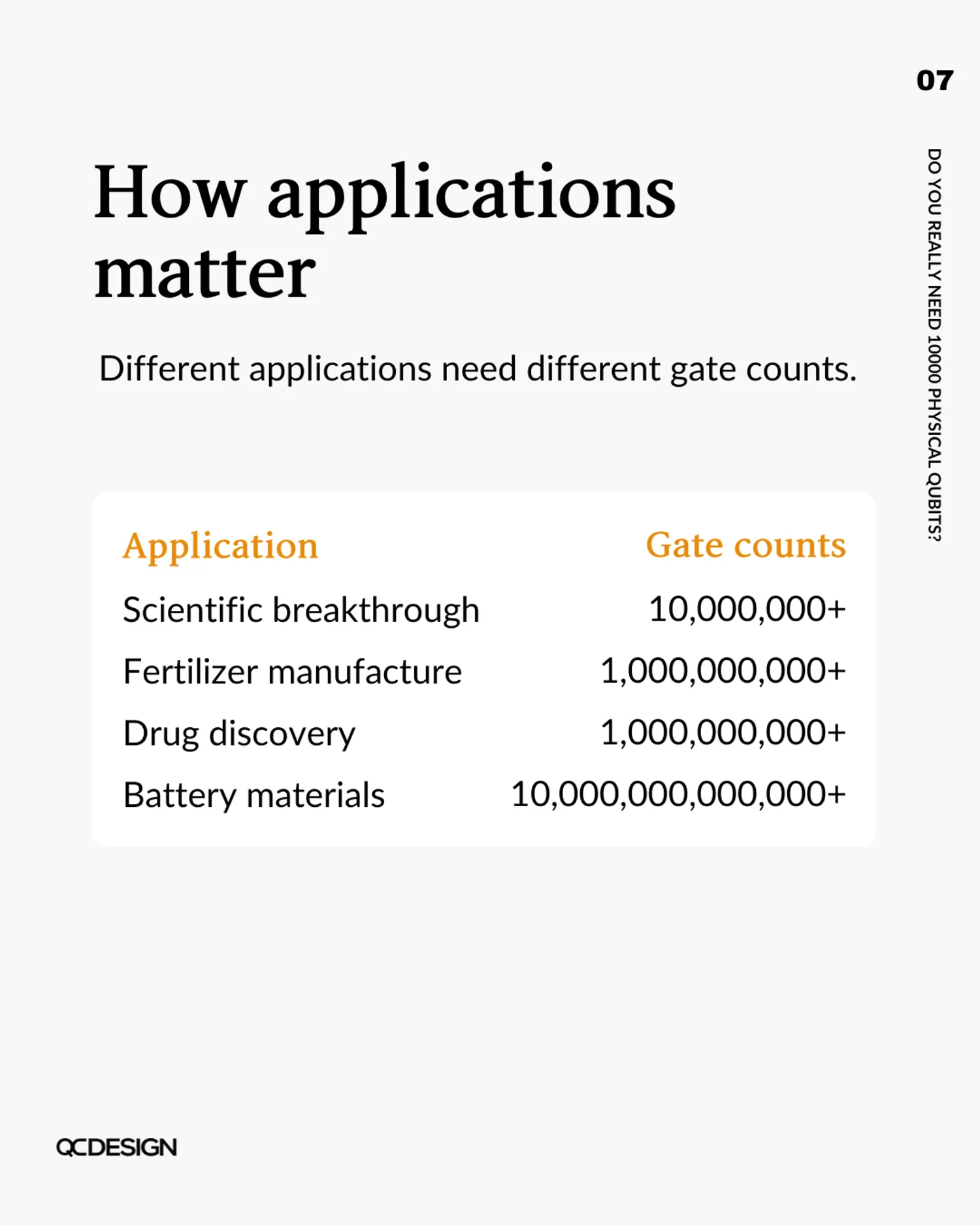
Different applications need different gate counts. Here are some examples:
| Application | Gate counts |
|---|---|
| Scientific breakthrough | 10,000,000+ |
| Fertilizer manufacture | 1,000,000,000+ |
| Drug discovery | 1,000,000,000+ |
| Battery materials | 10,000,000,000,000+ |
For a given application, the error per gate must be under 1 in roughly 10 times the gate count. For example, for 10,000,000 gates, the error per gate should be under 1 in 100,000,000. This tells us the logical error rate needed on the threshold plot (see blue arrow below).
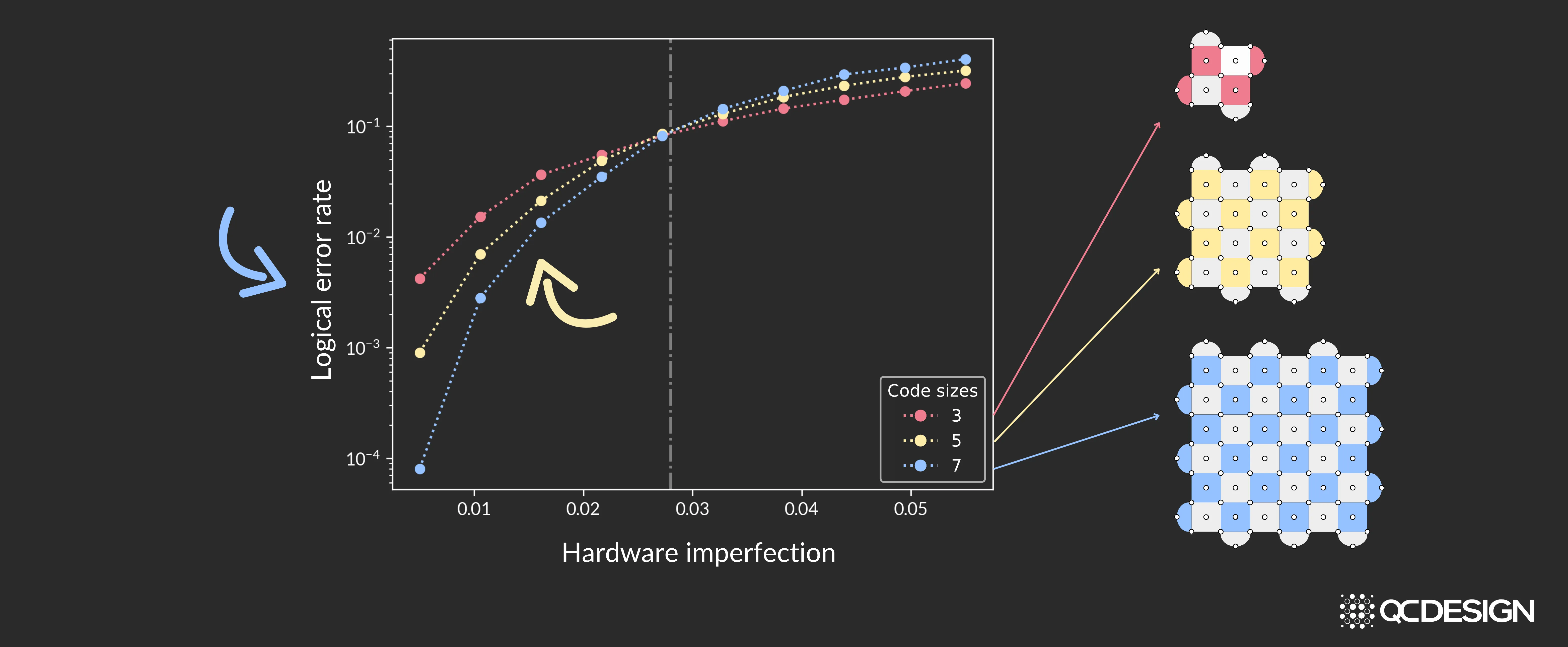
If an application needs more gates, it needs lower logical error rates, which (remember the different curves?) means we need a larger logical qubit (see yellow arrow above).
The imperfections in your system
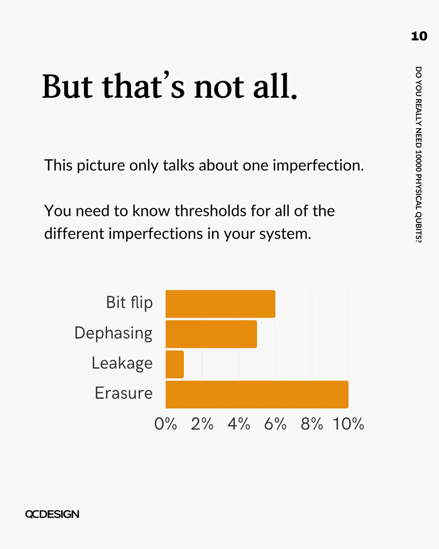
This picture above only talks about one imperfection, but you need to know the thresholds for all of the different imperfections in your system. As we explore in Not all errors are equal, different error types such as bit flip, dephasing, leakage, and erasure each have a different threshold.

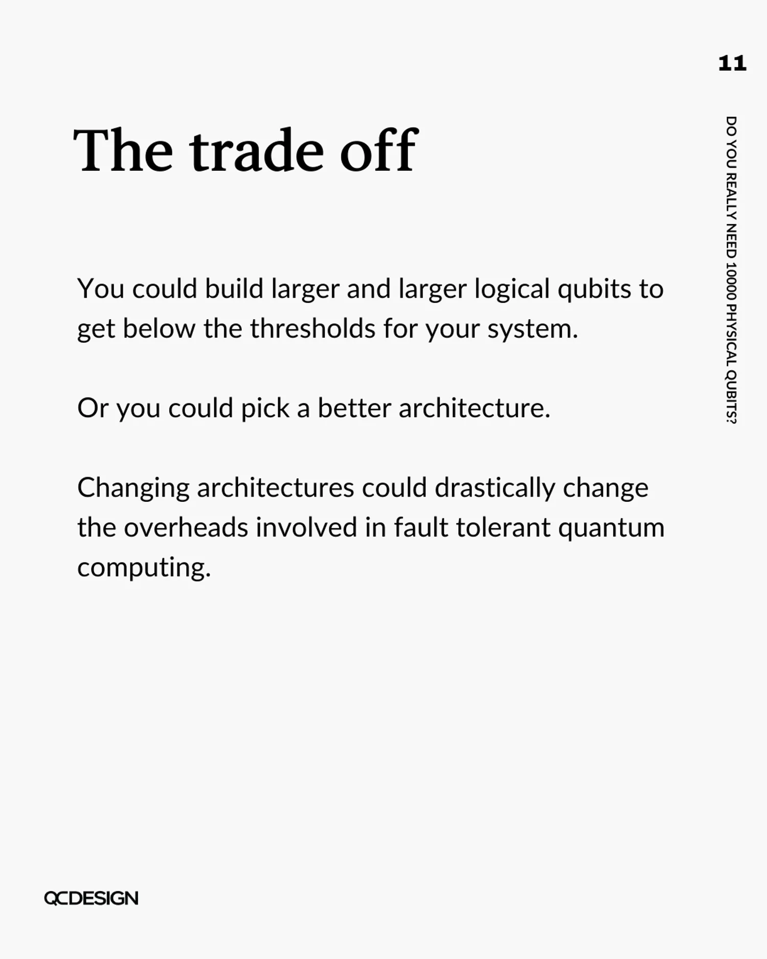
The trade off
You could build larger and larger logical qubits to get below the thresholds for your system, or you could pick a better architecture.
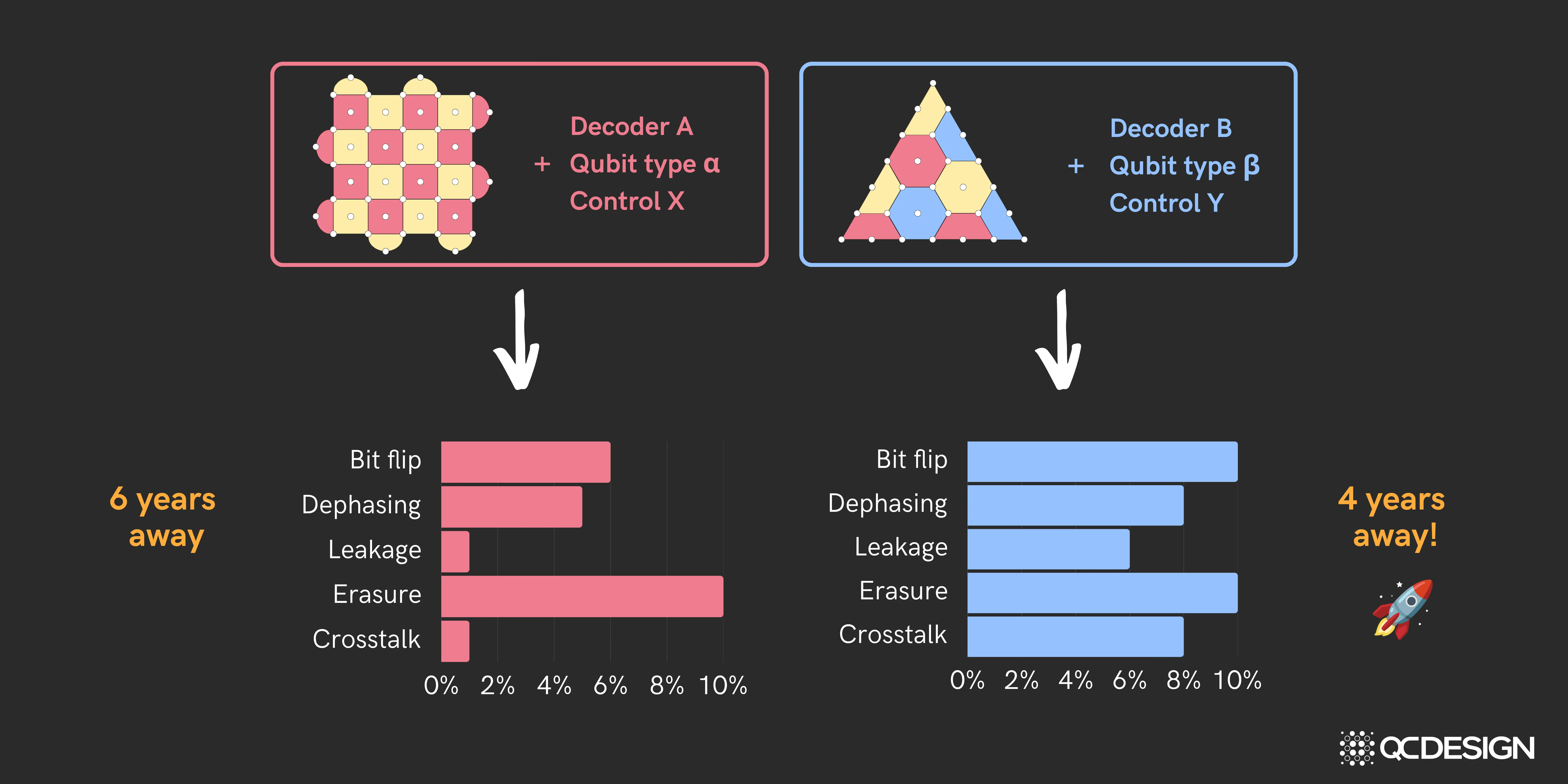
Changing architectures could drastically change the overheads involved in fault tolerant quantum computing. But how do you know which one to choose?
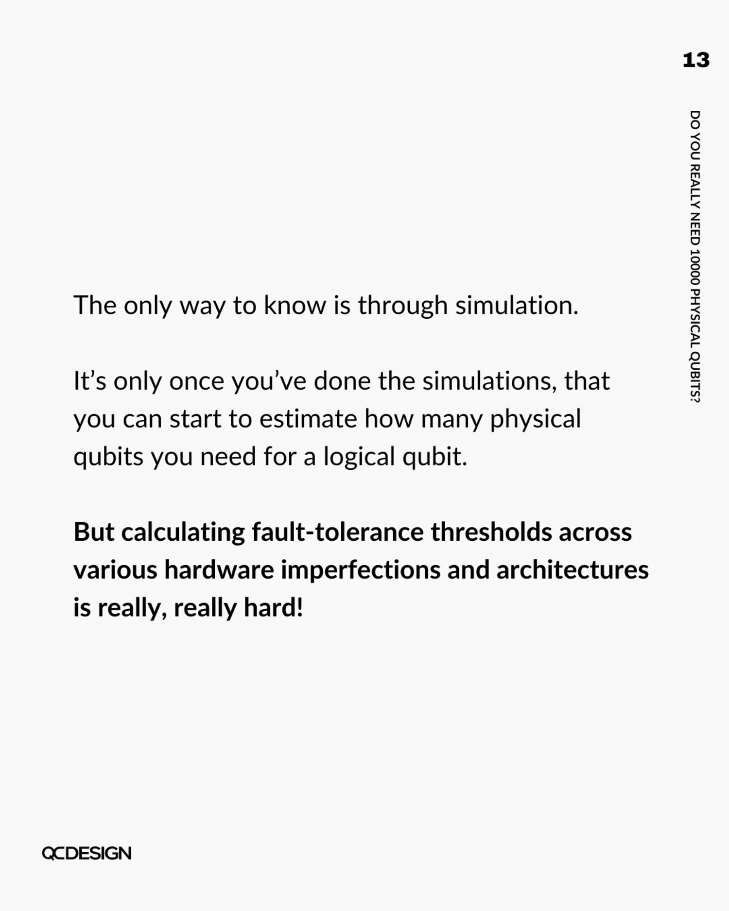
The only way to know is through simulation, and it’s only once you’ve done the simulations that you can start to estimate how many physical qubits you need for a logical qubit. Calculating fault tolerance thresholds across various hardware imperfections and architectures, though, is really, really hard.
How Plaquette helps
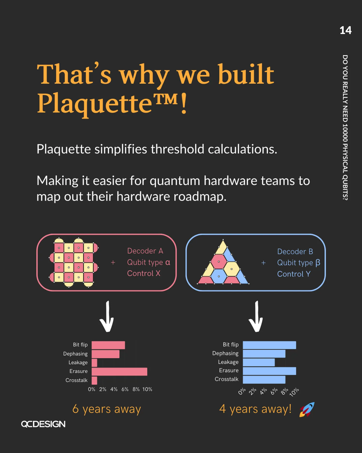
Plaquette simplifies threshold calculations, making it easier for quantum hardware teams to map out their hardware roadmap. As the figure above shows, the right choice of architecture can make a significant difference.
To find a threshold, Plaquette runs simulations across a range of error rates and code sizes, computes the logical error rate for each, and identifies the point below which a bigger logical qubit means fewer errors. It then plots the threshold so hardware teams can read it off directly.
A simulation is only as useful as how closely its error model matches your real hardware. Plaquette is built to capture a wide variety of hardware imperfections and to take in your device’s own characterized noise, so the thresholds you calculate reflect your actual system.
If you’re curious how Plaquette can work for your platform, get in touch and we can share a demo.
Not ready yet? You can also join our practitioners mailing list to be notified when we release new features or publish technical content like this.


This post was originally published in October 2025 and updated in June 2026.