How Plaquette Works In Practice

How Plaquette helps quantum hardware manufacturers design fault tolerant quantum computers. #

In our last post, we looked at the theory behind logical qubits and threshold behavior. In this post, we will focus on questions Plaquette helps answer, and show how those questions translate into logical error rates and threshold plots. With that context in mind, let’s first look at how Plaquette is actually used in practice.

Most people use Plaquette through Python in a Jupyter Notebook. Under the hood, Plaquette itself is written in C++ and optimized for performance, but Python is the layer that fits naturally into how hardware teams already work. It makes it easy to connect Plaquette to tools like Qiskit, as well as to internal codebases, without getting in the way of performance. This setup also makes it straightforward for hardware teams to plug in their own error models and circuits, and to generate logical error rates and threshold plots as part of their existing workflows.

In this post, we won’t dive into the code, but we’ll look at the kinds of calculations and questions a Plaquette user might be interested in studying.

Plaquette Workflow #

Before we do that, let’s first look at the full workflow Plaquette is designed to support. The figure below summarizes that workflow at a high level.

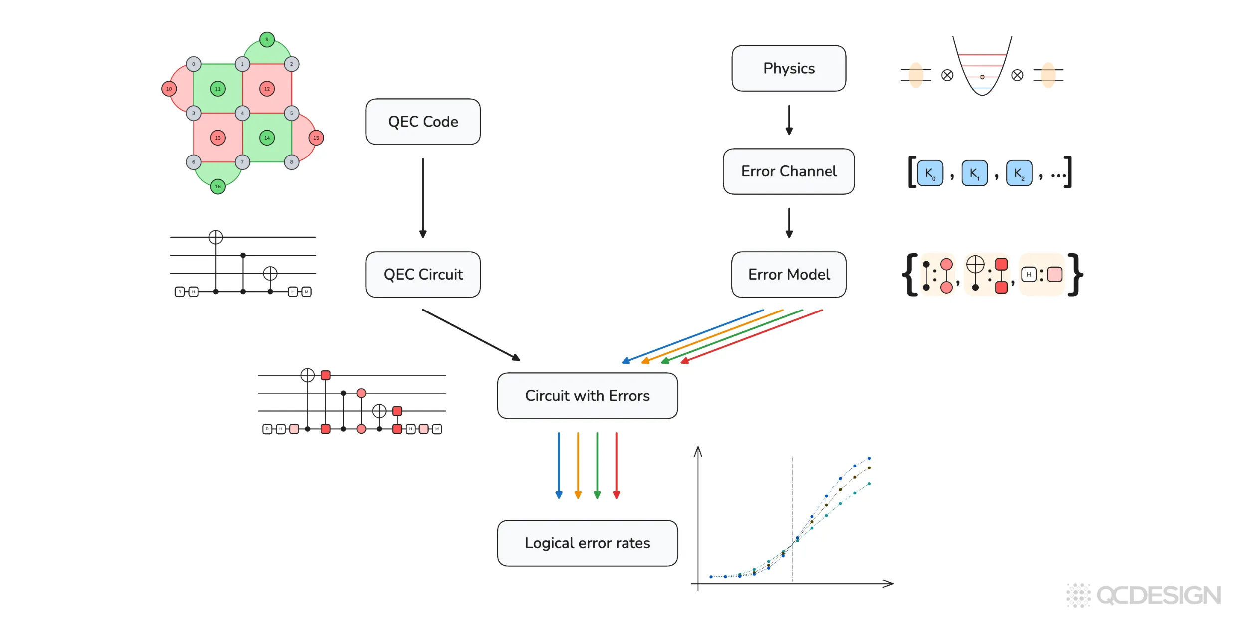
On one side, you start with a quantum error correction (QEC) code, which defines the structure of the logical qubit and produces a concrete QEC circuit. On the other side, you start from the physics of the hardware, which determines the error channels and the error model that specifies where and how errors act in that circuit.

These two pieces are combined to form a circuit with errors: a noisy implementation of the error-correction protocol that reflects both the code and hardware. Plaquette then simulates this circuit to estimate logical error rates. Repeating this across different physical error rates and code sizes produces the threshold plots used to compare different architectures.

The rest of this post unpacks each step in this pipeline, starting with how error correction codes are defined in Plaquette and working through error models, simulators, and finally logical error rates and thresholds.

Error correction code #

Recall from our previous post that a quantum computing architecture is defined by four things: (1) error correction code, (2) error decoding, (3) qubit definition, and (4) qubit control. So here, we first need to start with defining an error correction code.

Plaquette has a library of error correction codes that aims to include every error correction code that exists in the literature. Examples include:

• Shor code
• Repetition code
• Generalized bicycle code family from polynomials on a ring
• Bacon–Shor code
• Subsystem surface code
• Hypergraph product code
• Five-qubit code
• Subsystem repetition surface code
• Hypergraph product code from a random classical code
• Steane code
• Classical Hamming code (used to construct CSS codes)
• Lifted product code
• Planar code
• Generalized bicycle code
• Multivariate bicycle code
• Rotated planar code
• Generalized bicycle code from polynomials

For our example, we’ll stick to the simple repetition code. We do so by selecting the repetition code from the library and specifying that we want three qubits. Plaquette then generates the error correction circuit for this code:

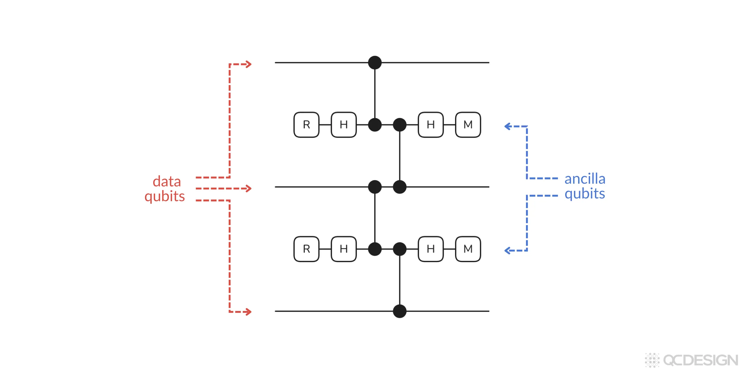
In the circuit above, you can see data qubits that contain the quantum information and ancilla qubits, which talk to these data qubits to find and correct the errors.

Say we want to study the effect of errors in this circuit. To do that we have to define two things: error models and error channels.

Error models #

An error model tells Plaquette where errors can occur in a circuit. Those locations can take many different forms. For example, an error might be applied before every round of error correction, after every round of error correction, or whenever a gate is applied to a particular qubit or set of qubits, causing the others to experience idling errors.

Idling errors act directly on qubits and are typically used to model what happens when nothing is being done to them. You can think of this as the effect of the surrounding environment on individual qubits.

Another important class of errors is tied to gates themselves. In this case, an error is applied after each gate operation. For instance, after a single-qubit gate like a Hadamard, you might apply a single-qubit error, while after a two-qubit gate like a CNOT, you might apply a different two-qubit error. These errors are used to model imperfect gate operations, which arise either because control pulses are imperfect or because the exact target unitary can’t be realized in practice.

Qubit-level errors and gate-level errors are the main types of errors of interest in error correction. Plaquette supports modeling both types.

In architectures that rely on moving qubits, error models may also include shuttling errors, where the error rate increases with the distance a qubit is transported.

In Plaquette, error models are specified as Python dictionaries. They can be selected from a pre-existing set of common error models, defined manually, or constructed from several convenience functions within Plaquette.

Let’s consider two examples.

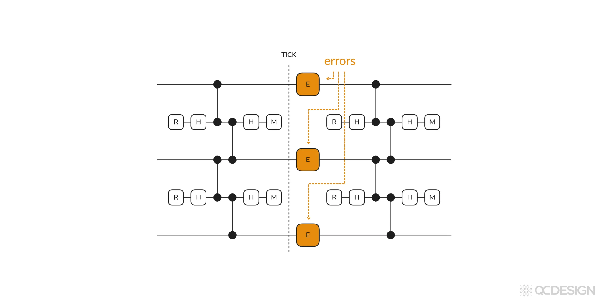
Example 1: Idling errors #

Let’s imagine we want to study a case where errors happen whenever the data qubits are idling (basically just sitting around). We can set this by selecting the pre-defined idling option. Plaquette then generates the following circuit:

We can also consider more interesting cases.

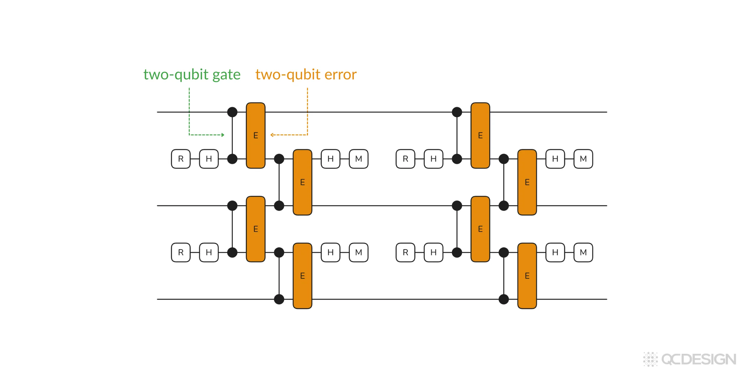
Example 2: Errors on two-qubit gates #

For this example, let’s take a look at the situation where every time a two-qubit gate occurs in the circuit, it experiences a two-qubit error.

As above, we specify a three-qubit repetition code, but now we define the error model as a dictionary pair containing the CZ gate and a two-qubit error channel. Plaquette generates this circuit:

Once you have an error model, the next step is to define the error channels for the errors “E” in your model.

Error channels #

Most hardware teams describe their error channels using Kraus operators, since that’s what tends to come out of their internal noise and device simulations. These operators are standard constructions that apply broadly across hardware platforms, and they are the same kinds of operators used in well-known threshold experiments. Plaquette is set up to take those outputs directly. If you already have a way of modeling your errors internally, you can usually plug that straight into Plaquette and let it do the rest.

At the same time, Plaquette is extremely general when it comes to error channels. As long as you can specify your error channels in one of the standard mathematical forms (Kraus operators, Pauli transfer matrices, Hamiltonians, or Lindbladians) Plaquette can work with them. This holds true for most of the important system configurations: qubits, qudits, and qubits coupled to other ancillary qubits or qumodes.

Below, we’ll look at two classes: coherent errors and incoherent errors.

Coherent Errors #

Let’s start with a simple example: over-rotation errors. Suppose a gate consistently rotates a little too far compared to what we intended. We can model that over-rotation using a unitary operator:

$$U = e^{-i\theta(\hat{Z} + \hat{X})}$$

where the size of the error is set by a small parameter $\theta$. In this case, the error is fully described by a unitary transformation. That’s what makes it a coherent error.

Coherent errors are important to many platforms, but they’re not the only kind of error. Another class of errors are known as incoherent errors. Noise due to incoherent errors can’t be described with unitary operations as above.

Leakage errors #

A common and important example of incoherent errors arising in several hardware platforms is leakage. Imagine a state that starts in the computational subspace (the states we call ‘0’ and ‘1’) but can temporarily leave that subspace and occupy higher energy levels like ‘2’ or ‘3’, before possibly coming back again.

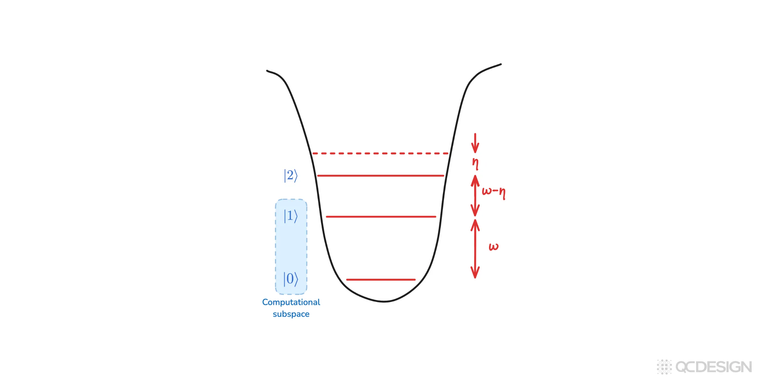
As mentioned above, incoherent errors can’t be specified using unitary operators. Instead, they can be described using Kraus operators. For the leakage channel, the Kraus operators are:

$$K_1 = \sqrt{p_t}\left(|02\rangle\langle11| + |11\rangle\langle02|\right),$$ $$K_0 = \sqrt{I - K_1^\dagger K_1}$$

Another important source of incoherent error comes from coupling to additional degrees of freedom. For example, in trapped-ion systems, qubits are coupled to motional modes.

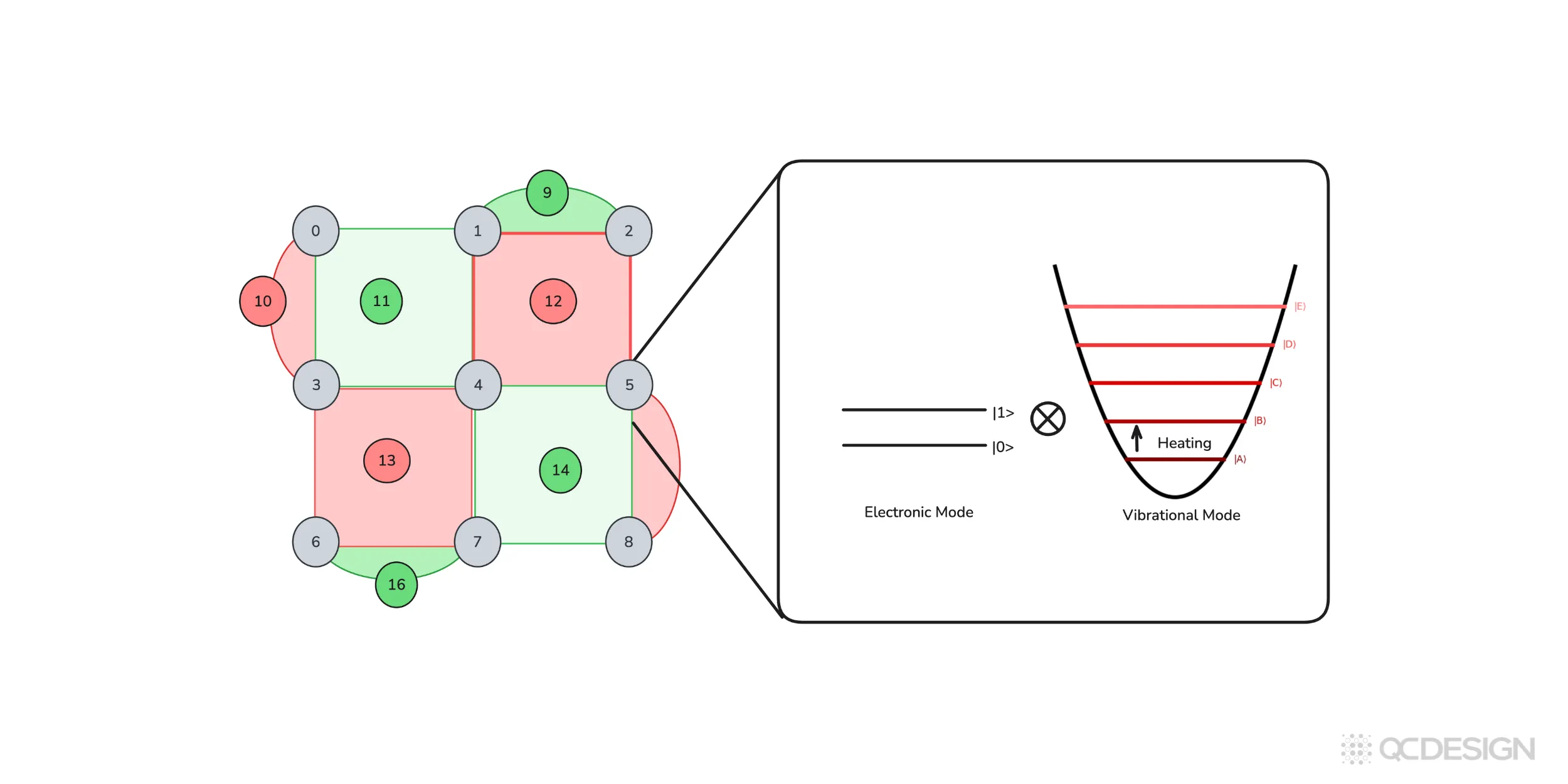
Heating of those modes can introduce errors even if the internal qubit states are well controlled. Similar effects appear in neutral-atom platforms, where motional degrees of freedom again play a central role. In these cases, the system you care about is not just a qubit, but a qubit plus an additional mode evolving together. Plaquette is designed to handle these kinds of situations as well.

Next we need to choose a simulator.

Simulators #

Plaquette has access to five simulators. Different simulators are better suited to different kinds of error models and different system sizes, and there’s a trade-off between how fast the simulation runs and how much detail you can include in the noise.

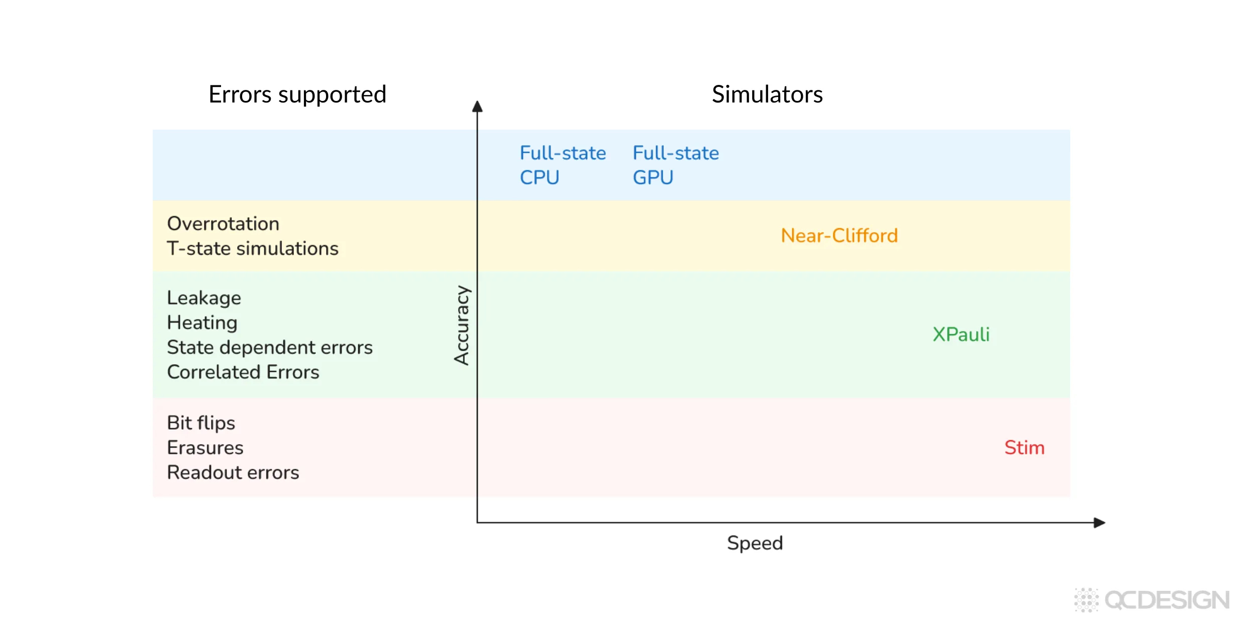
The faster stabilizer-based simulators (Stim and XPauli) are what you’d use for large threshold studies, where you might need millions of shots. The more general simulators (Near-Clifford and Full-state) can capture non-Pauli and other realistic effects, but they’re heavier computationally.

Let’s look at what this means in practice, starting with the simplest case.

Clifford errors on qubits #

The simplest case is when your error model is limited to Clifford errors (e.g. discrete X and Z Pauli errors, or stochastic Pauli noise) and they act only on two-level systems. There’s no leakage, no higher levels getting involved, no coupling to ancillary modes. In that regime, you should just use Stim. It’s very well matched to exactly this kind of problem and extremely fast. Since Stim is one of the backends supported by Plaquette, you can plug it in directly.

Coherent errors on qubits #

Now let’s consider slightly more complicated errors: coherent over- or under-rotation. The gate is still acting on a two-level system, but the error itself is no longer Clifford. This is what happens when a control pulse is slightly too long or too short.

At that point, you have a choice. One option is to apply Pauli twirling. This is an approximation where you deliberately discard the coherent part of the error channel and replace it with an effective stochastic Pauli error. Once you do that, you can still use Stim. There are strong reasons why people in quantum error correction think this is a good approximation, but it is still an approximation.

In some cases, especially for smaller codes, or for particular forms of coherent error, Pauli twirling can give misleading results. In those regimes, using a stabilizer-only simulator like Stim is no longer a good approximation, and it makes sense to switch to something more general, such as the Near-Clifford simulator.

How expensive this simulation becomes depends on how far the circuit is from being Clifford. If the non-Clifford component is small, the overhead is manageable. If it’s large, the number of samples you need grows quickly. Plaquette can estimate this cost in advance. For the example where $\theta = 0.015$, Plaquette tells us that we need on the order of ten million samples to achieve a 1% error bar on the logical error rate.

To see how the simulators compare, we can simply run ten million shots with each backend.

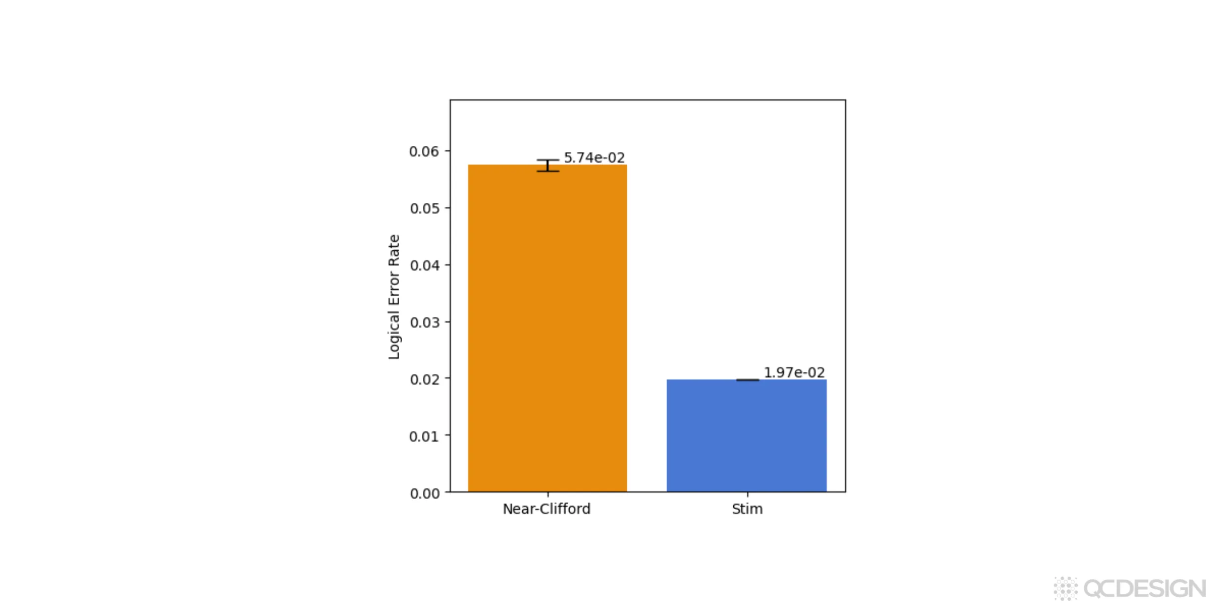
The near-Clifford simulator gives a logical error rate of about 6%, while the Stim backend gives a value closer to 2%. The key point is that the near-Clifford result is exact for this coherent error model, whereas the Stim result relies on an approximation. In this case, that approximation underestimates the logical error rate by roughly a factor of three.

This already highlights something important: if you care about getting the logical error rates right in the presence of coherent, non-Clifford noise, you need to use a simulator that can actually represent that noise. Otherwise, you risk drawing the wrong conclusions about how well your hardware or error-correction scheme is really performing.

The near-Clifford simulator is known to be theoretically exact and unbiased, but that accuracy comes at a cost. It can require a large number of shots, and the required number depends very sensitively on how non-Clifford the circuit is. A circuit with a few strongly non-Clifford errors, or a circuit with many weakly non-Clifford errors, can quickly become expensive to simulate. When you do run it, though, the result is an accurate and unbiased estimate of the logical error rates.

Errors involving more than 2 levels #

So far, everything we’ve talked about has assumed a two-level system. But in many real devices, you can have leakage into higher energy levels, heating events in trapped ions, or additional degrees of freedom like valley states in spin qubits. Once that happens, simple Clifford simulations are usually no longer enough.

In some special cases, you can still get away with a Clifford simulator. For example, if a qubit leaks out of the computational subspace and never comes back (it’s effectively lost and no longer participates in the circuit) then you can sometimes just discard it and keep going. In those situations, using Stim can still give you the right answer, and it will do so very quickly.

But as soon as you want more accurate modeling, especially when population can leave the computational subspace and then come back, you need something more general. One option is to use a full-state simulator on qudits. This is very accurate, but also very slow. If you’re working with qudits of dimension four or five, you quickly run into hard limits, on the order of a few tens of qudits, because of the exponential scaling. Using Plaquette’s GPU backend can push that boundary further, but the exponential wall is still there.

This is where Plaquette’s XPauli simulator comes in. XPauli is designed to sit between these two extremes. Inside the computational subspace, it uses a Clifford-style simulation, which is efficient and scales polynomially, much like Stim. Anything that happens outside the computational subspace is treated as a classical jump process. Coherences are discarded when the system leaves the qubit subspace, and population can later return.

That “coming back” part is important. Standard Clifford simulators can’t model that at all. XPauli can. This makes it particularly useful for modeling leakage in superconducting qubits, or heating processes where a motional mode is excited above the ground state and then relaxes again.

From a performance point of view, XPauli is still very fast (typically only an order of magnitude slower than Stim) and it scales polynomially. In many realistic leakage scenarios, it turns out to be almost as accurate as a full-state simulation, while being orders of magnitude faster.

We can run the same comparison for leakage errors. In this case, we specify the leakage channel directly by entering the Kraus operators in matrix form, set $p_t = 0.2$, and assume four leakage levels. Other than that, the workflow is essentially unchanged. We run the same circuit using the full-state, XPauli, and Stim simulators and compare the resulting logical error rates.

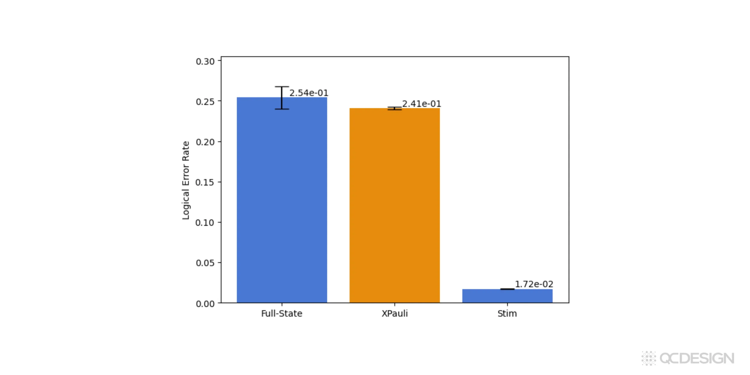
The full-state simulator gives the exact result and the XPauli simulator agrees with it within error bars. At the same time, XPauli runs much faster and produces significantly smaller statistical uncertainties than the full-state simulation.

Stim, on the other hand, runs even faster, but it severely underestimates the logical error rate in this leakage scenario. This is exactly the kind of situation where treating everything as a two-level system breaks down: population leaves the computational subspace and later returns, and that dynamics simply isn’t captured by a Clifford-only model.

Taken together with the coherent-error example above, this highlights an important point. Plaquette’s XPauli and near-Clifford simulators let hardware teams access a level of accuracy that isn’t available with open-source Clifford simulators like Stim, while still avoiding the steep cost and scaling limits of full-state simulations. In practice, they make it possible to study realistic error models at system sizes that would otherwise be out of reach.

Ongoing development #

These are the simulators Plaquette supports today. That said, fault-tolerant quantum computing is moving quickly, and new simulation methods keep appearing. We’re actively developing new simulators ourselves, and we also track what’s happening across the broader fault-tolerance community.

XPauli is one example of that. It’s a simulator we developed to go beyond what was previously available. As far as we’re aware, it’s the only approach (published or unpublished) that can handle both high-energy leakage levels and additional degrees of freedom, like vibrational modes, within a single framework, including combinations of the two.

As new simulation techniques emerge, we continue to add them to Plaquette. The goal is to make sure users have access to the right tools as the field evolves, rather than locking them into a single approximation or model.

Threshold plots #

The examples above represented a single point on a threshold plot. But Plaquette also makes it very easy to make full threshold plots and identify thresholds.

Following the same workflow as above, but with an additional line of code, we can find all the logical error rates involved. We can then plot the logical error rates on a nice threshold plot and basically use that for, finding our thresholds.

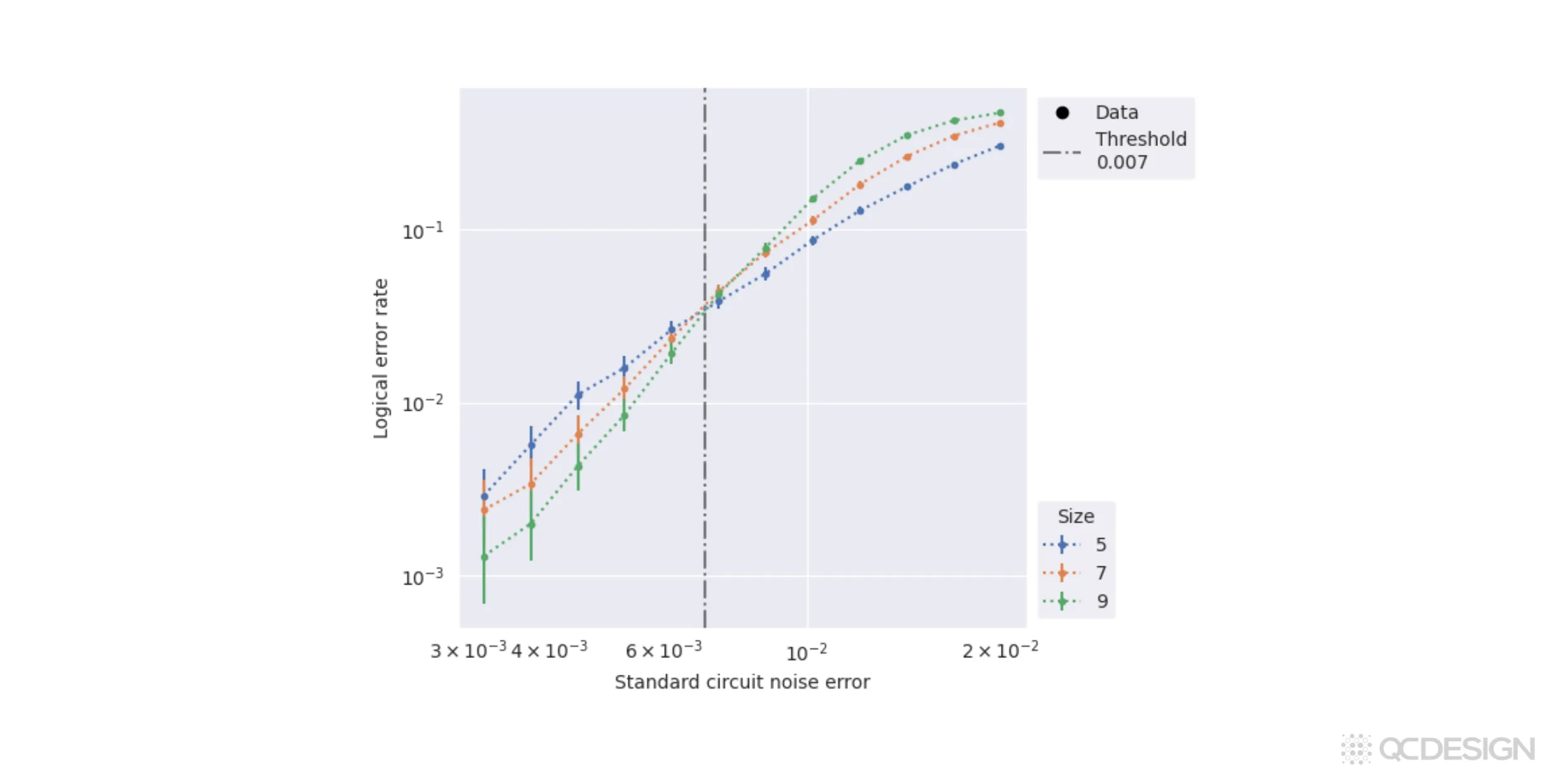
In this case, we see that the threshold is close to 0.67% for standard circuit noise.

We hope these examples give you a taste of how Plaquette combines accuracy, speed, and ease-of-use, in a way not available anywhere else, to help hardware manufacturers get the most out of their hardware systems.

Next steps #

If you’d like to do a deeper dive into how Plaquette works for your own platform, get in touch and we can share a demo.

Not ready yet? You can also join our practitioners mailing list to be notified when we release new features or publish technical content like this.